
Computing with chance
The exact statements and the proofs of what the film showed.
How many samples does it take to be right, and how do you prove it?
In 1946, the mathematician Stanislaw Ulam wonders what chance a game of solitaire has of ending in a win. The exact calculation is out of reach; playing a hundred games and counting is not. This chapter turns that sickbed idea into a method of computation, and above all into a verifiable method: we will be able to say how many samples are needed, and with what guarantee.
The chapter follows the film of session 1, “Computing with chance”: Ulam’s problem (Section 1.1), the law of large numbers (Section 1.2), computing an area (Section 1.3), the Monte Carlo estimator and its two textbook cases, the call option and an insurer’s ruin (Section 1.4), the central limit theorem and the confidence interval (Section 1.5), dimension and rare events (Section 1.6).
1.1 Ulam’s problem#
Recovering from encephalitis, in Los Angeles, Ulam plays Canfield solitaire, a card game for one player with 52 cards. He tries to calculate the probability that a deal comes out successfully; but the number of possible orders of the deck is 8.07, and no enumeration is conceivable. He then thinks of laying the cards out “say one hundred times” and counting the successes (Eckhardt 1987). With John von Neumann, he immediately sees that the same idea applies to neutron diffusion at Los Alamos: a problem with countless dimensions, in which an equation can be replaced by a sequence of random operations. The code name, “Monte Carlo”, is suggested by Nicholas Metropolis, in memory of an uncle of Ulam’s who borrowed money from relatives to go gambling at the casino (Metropolis 1987); the first paper on the method appears in 1949 (Metropolis and Ulam 1949).
The question to keep in mind: how many games would Ulam have to play to know his chance to within 1%? It is answered in Section 1.5.
1.2 A probability is a proportion#
1.2.1 The setting#
We work on a probability space . A real random variable is a measurable function from to ; its distribution is the image measure .
Random variables form a sample (or i.i.d. sequence) with distribution if they are independent and all have distribution . To simulate is to produce, on a computer, realisations of such a sample.
A probability is an expected value: for every event , , and if . Estimating a probability therefore means estimating the mean of a variable that equals 1 or 0: the proportion of successes among trials.
1.2.2 Ten tosses: the exact result becomes rare#
In ten tosses of a fair coin, the number of heads follows the binomial distribution . There are sequences out of 1,024 that give exactly five heads: only 24.6%. Six heads and four tails, or the reverse, happens 41% of the time. The video opens on six heads and four tails: nothing unusual.
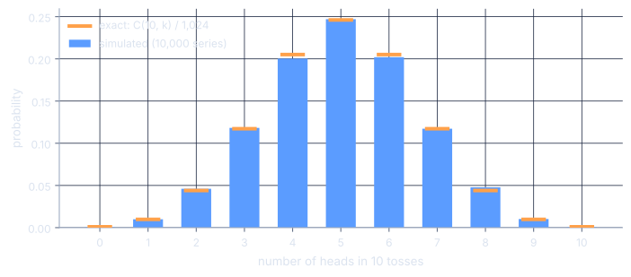
The simulation of 10,000 series gives 2,470 series with five heads, that is 24.70%; the blue bars land on the orange marks. The larger grows, the more improbable “exactly half” becomes, but the more certain “about half” becomes: that is what the law of large numbers says.
1.2.3 The law of large numbers#
If , then for all , .
Proof
The inequality holds pointwise; take expectations.
Let be a sample with , and . Then the sample mean satisfies, for all ,
Proof
By linearity, ; by independence, the variances add up: . Apply Proposition 1.1 to .
The weak law says that the error is rarely large; the strong law says that the sequence of estimates, the one we see settling down on a screen, converges.
If is a sample with , then almost surely.
Proof
We prove the statement under the stronger assumption , which is enough for this whole course; the general case requires a truncation argument (Etemadi 1981; Durrett 2019). Replacing by , we may assume . Write . When is expanded, the terms that contain some to the power 1 have zero expectation by independence; what remains is Markov’s inequality gives , the general term of a convergent series. By the Borel–Cantelli lemma, almost surely from some index onwards. We conclude by taking , (a countable intersection of almost sure events).
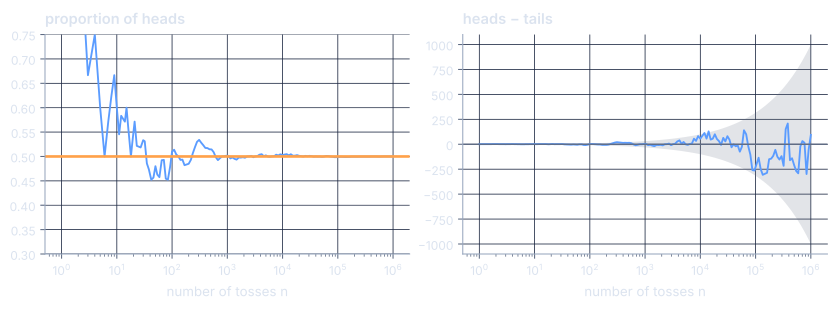
Applied to , the strong law says that the proportion converges to : a probability is a proportion, in the limit. In the video, the proportion of heads is 50.28% after 10,000 tosses and 50.005% after a million.
Proof
Chance does not even out. The gap between the number of heads and the number of tails, , has mean zero and variance : it does not tend to 0, it typically grows like (in the video, it is +94 after a million tosses). By the central limit theorem (Section 1.5), . But : divided by , the gap is crushed and the proportion converges. The “gambler’s fallacy”, the belief that after a run of tails heads is “due”, confuses these two scales: the coin has no memory; deviations are not corrected, they are diluted (Tversky and Kahneman 1974).
1.2.4 Simulating on a computer#
A computer does not toss coins: it computes a sequence of numbers by a deterministic recursion, whose statistical properties imitate those of a uniform sample. NumPy uses the PCG64 algorithm (O’Neill 2014): np.random.default_rng(seed) creates a generator, and the same seed gives back the same sequence. The code from the video, run here:
rng = np.random.default_rng(2)
faces = rng.random(1_000_000) < 0.5
print(faces.mean())0.500047Everything else is built from the uniform distribution. The basic tool is the inversion of the cumulative distribution function.
Let be a cumulative distribution function and its generalised inverse. If is uniformly distributed on , then has cumulative distribution function .
Proof
is non-decreasing and right-continuous, so the set is a closed interval . Hence , and .
For the exponential distribution with mean , and . These are the samples we will use in the next chapter for the insurer’s “twin”: two different distributions obtained from the same uniforms. For the normal distribution, NumPy uses an algorithm faster than inversion (rng.standard_normal).
1.3 An area can be counted#
Let be uniform on the square . For every measurable subset of the square, . With the quarter disc , of area : where is the number of points, out of , that land in the quarter disc. This is the strong law of large numbers applied to an indicator: an area can be counted.
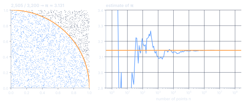
Of the video’s 3,200 darts, 1,582 land below the diagonal (49.4%, for an area of ½) and 2,505 in the quarter disc: 3.131. With , and points, the estimate is 3.1256, 3.1405 and 3.1415: each digit costs about a hundred times more points than the previous one. The reason is given in Section 1.5.
More generally, every integral over the unit cube is an expected value: with uniform on . This is the starting point of Monte Carlo numerical integration.
Buffon poses the following problem in 1733, and publishes it in 1777 (Buffon 1777): a needle of length falls at random on a plank floor whose cracks are apart; what is the probability that it crosses a crack? Let be the distance from its centre to the nearest crack, uniform on , and its angle with the cracks, uniform on , the two being independent. The needle crosses a crack if and only if , hence Laplace turns the question around in 1812 (Laplace 1812): drop needles, count the crossings, and estimates . (A famous experiment of 1901 claimed six correct decimal places with 3,408 needles: a result almost certainly obtained by stopping at the right moment, which is exactly what a confidence interval forbids.)
1.4 An expected value is an average#
1.4.1 The Monte Carlo estimator#
Let be a random variable with values in , measurable with , and . For a sample with the same distribution as , the Monte Carlo estimator is
This is the formula from the video, read symbol by symbol: is the outcome of chance (the die, the coin, the price of a share tomorrow), is what we look at in that outcome (the number showing, a gain, a loss), is the long-run average we are after, are the computer’s samples; we add them up and divide by . The average we want is roughly the average of what we observe by simulating.
- is unbiased: ; it is strongly consistent: a.s. (Theorem 1.2).
- If moreover and , then : the typical error (the standard deviation of the estimator) is .
Proof
Linearity of expectation, the strong law applied to the , which are i.i.d. and integrable, and additivity of the variance for independent variables.
For a fair die, , a value that no roll ever gives; the average of 10,000 simulated rolls is 3.5088.
def monte_carlo(Y):
    """Estimate and half-width of the asymptotic 95% confidence interval, from the samples Y = f(X_i)."""
    Y = np.asarray(Y, dtype=float)
    return Y.mean(), 1.96 * Y.std(ddof=1) / np.sqrt(len(Y))
1.4.2 Finance case: the call option#
A European call option (a call for short) with strike and maturity gives the right, but not the obligation, to buy the share at time at the price . Its payoff at maturity is . Arbitrage pricing theory (see the stochastic calculus course) shows that its price today is the expected value of the discounted payoff under the risk-neutral probability : In the Black–Scholes model (Black and Scholes 1973; Merton 1973), the price follows a geometric Brownian motion and, under , with , where is the risk-free rate and the volatility (the annual standard deviation of returns). The price is an expected value: it can be simulated (Boyle 1977). For this simple case, we also know the exact value, which will serve as the judge.
If with and , then
Proof
. On the one hand, . On the other hand, writing for the density of , completing the square shows that ; hence with , that is, .
With and , we obtain , with and .
For , , , year, the judge is €10.4506. The following code simulates a million futures:
S0, K, r, sig, T = 100.0, 100.0, 0.05, 0.20, 1.0
rng = np.random.default_rng(1973)
Z = rng.standard_normal(1_000_000)
ST = S0 * np.exp((r - sig**2 / 2) * T + sig * np.sqrt(T) * Z)
prix, demi = monte_carlo(np.exp(-r * T) * np.maximum(ST - K, 0))
print(f"Monte Carlo: {prix:.3f} ± {demi:.3f}   |   Black–Scholes: {bs_call(S0, K, r, sig, T):.4f}")
Monte Carlo: 10.426 ± 0.029 | Black–Scholes: 10.4506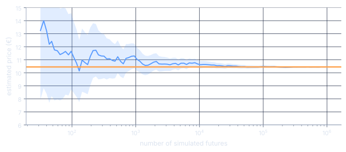
In the video, a million futures give €10.46 with a typical error of €0.015, against €10.45 for Black–Scholes. The point of simulation is not to recover a known formula: it is to keep working when there is no formula left (options on averages, on several assets, stochastic volatility models). The judge serves to validate the method in the case where it exists.
1.4.3 Insurance case: ruin#
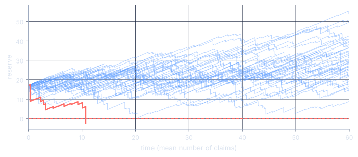
The Cramér–Lundberg model describes an insurer’s reserve: where is the initial reserve, the premium rate, a Poisson process with intensity (the claim times) and i.i.d. claim sizes with mean , independent of . The premium includes a safety loading : . The ruin probability is , once again the expected value of an indicator.
If the claim sizes are exponential with mean , then .
The proof (by a renewal argument, or with Lundberg’s exponential martingale) is classical (Asmussen and Albrecher 2010, chap. IV). It provides the orange judge of the video.
To simulate, note that the reserve can only fall below zero at the moment of a claim. Writing for the times between claims (exponential with parameter ), the reserve just after the -th claim is the random walk , and ruin is the event . We truncate the horizon at claims.
def ruine(rng, N, u, theta, n_sinistres=1000):
    """Cramér–Lundberg (λ = 1, Exp claims with mean 1, c = 1 + θ): ruin before n_sinistres claims, and final reserve."""
    R = np.full(N, float(u))
    ruinee = np.zeros(N, dtype=bool)
    for _ in range(n_sinistres):
        R += (1 + theta) * rng.exponential(1.0, N) - rng.exponential(1.0, N)
        ruinee |= R < 0
    return ruinee, R

ruinee, R = ruine(np.random.default_rng(1903), 10_000, u=17, theta=0.2)
p, demi = monte_carlo(ruinee)
print(f"simulated ruin: {p:.4f} ± {demi:.4f}   |   exact: {ruine_exacte(17, 0.2):.4f}")
simulated ruin: 0.0501 ± 0.0043 | exact: 0.0490These are exactly the samples used in the video (same seed, same order): 501 ruins out of 10,000, that is 5.01% ± 0.43%, while the exact value is 4.90%.
Proof
The truncation bias can be measured. The estimator targets , not . By the strong Markov property, the difference is , which we estimate on the same paths thanks to the exact formula for : we find about , negligible compared with the statistical error. Predict, simulate, verify: even the approximations of the algorithm can be checked.
1.5 How many samples?#
1.5.1 The result is itself random#
Three estimates of with 1,000 points each give 3.140, 3.204 and 3.128: the estimator is a random variable. Its distribution describes the error. The weak law gave a bound; the central limit theorem gives its shape.
Let be a sample with , and . Then
Proof
Let , the standardised variables, and . Since , we may differentiate twice under the expectation (dominated convergence): is of class , with , , , hence . By independence, the characteristic function of is .
Lemma. If are complex numbers of modulus at most 1, then (by induction on : ).
For fixed and , apply the lemma to and : Since , the characteristic function of converges at every point to that of , and Lévy’s continuity theorem (Durrett 2019, sect. 3.3) gives convergence in distribution.
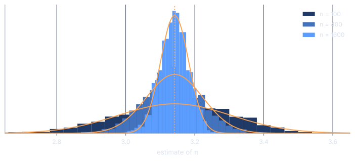
For the estimator of , one sample is , with standard deviation 1.642 where . The standard deviations measured over 2,000 repetitions in the video are:
| points | measured standard deviation | predicted |
|---|---|---|
| 100 | 0.1637 | 0.1642 |
| 400 | 0.0808 | 0.0821 |
| 1,600 | 0.0412 | 0.0411 |
| 10,000 | 0.0164 | 0.0164 |
Four times as many points halve the error; a hundred times as many points gain one digit. This is the golden rule of the method, and the reason why the digits of arrived so slowly in Section 1.3.
1.5.2 The confidence interval#
In practice is unknown: we replace it by the sample standard deviation, defined by , which converges almost surely to (strong law applied to the and to the ). The substitution is justified by the following lemma.
If in distribution and in probability ( a constant), then in distribution.
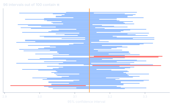
Under the assumptions of Theorem 1.4, for and , For , : this is the interval “estimate ”.
Proof
a.s., so in probability; by Lemma 1.2 and Theorem 1.4, in distribution. The event in question is ; the limit distribution puts no mass on the boundary , so .
1.5.3 The answer to Ulam#
For a proportion, . With games, the half-width of the 95% interval is therefore at most : with a hundred games, Ulam would have known his chance to within 9.8 percentage points, in the worst case. To get down to , we need Dividing the error by ten costs a hundred times more samples: the price of a digit.
Proof
A non-asymptotic guarantee. Theorem 1.5 is asymptotic. For variables bounded in , Hoeffding’s inequality (Hoeffding 1963) gives a guarantee that holds for every : . For Ulam (), an error of at most 1% with probability at least 95% is guaranteed as soon as , that is 18,445 games: the price of certainty is about twice the asymptotic price.
1.6 Why finance loves it#
1.6.1 Dimension#
To compute an integral over , one can also use a grid: points per axis, points in all. For a function of class , the midpoint rule has an error of (second-order Taylor expansion in each cell: the first-order term cancels out by symmetry). Monte Carlo has an error of order , regardless of . The grid wins in dimension 1, 2 or 3; it loses as soon as , and it becomes impractical well before that: ten points per axis in dimension 50 make points, the order of magnitude of the number of atoms in the Earth. This is the curse of dimensionality.
| dimension | 1 | 2 | 3 | 10 | 50 |
|---|---|---|---|---|---|
| points in a grid with 10 points per axis | 10 | 100 | 1,000 | ||
| Monte Carlo error for samples |
In finance, the dimension is the number of random quantities in a scenario: a path of 48 steps has 48 dimensions, a portfolio of 50 shares over 12 months has 600. This is the real reason for the method’s success. The constant , on the other hand, can depend on : that is the subject of session 2 (reducing it) and of challenge 2 of the practical.
1.6.2 The Achilles’ heel: the rare event#
For a small probability , the relative error of is which depends only on the number of events observed. For a relative error of 10%, about a hundred events must be observed, hence samples. Picture an insurer with enough reserves for ruin to happen, someday, only about once in two hundred: in the model of Section 1.4, an initial reserve gives an exact ruin probability of 0.475%. That is the order of magnitude of the Solvency II directive, which calibrates an insurer’s capital so that its ruin within one year has only a 0.5% chance of happening (Parlement européen et Conseil 2009); but these are two different probabilities: the directive looks at a single year, the model at the whole future. With 100 simulations, no ruin at all is observed with probability 0.62. With 1,000 simulations, the video observes 6: 0.6% ± 0.5%, which tells us almost nothing; it takes a hundred thousand to obtain 0.49% ± 0.04%. Session 3 will teach us to aim where it counts.
1.6.3 Historical landmarks#
Fermi was already practising statistical sampling in Rome in the early 1930s, without publishing; Ulam does not invent the idea, he marries it to the computer.
On 11 March 1947, von Neumann sends Robert Richtmyer, at Los Alamos, a plan for a statistical computation of neutron diffusion (Eckhardt 1987). The first simulations run on the ENIAC in the spring of 1948; Klára Dán von Neumann writes most of the programs (Haigh et al. 2014). The first paper, “The Monte Carlo Method”, appears in 1949 (Metropolis and Ulam 1949). In finance, Phelim Boyle introduces simulation into option pricing in 1977 (Boyle 1977).
1.7 What to remember#
- A probability is a proportion: almost surely (strong law of large numbers); chance does not even out, it gets diluted.
- An expected value is an average, and an average can be simulated: , unbiased, with variance .
- The error shrinks like : one digit costs a hundred times more samples; always report the estimate with its interval , which contains the true value 95 times out of a hundred.
The program from the video, in seven lines, run here:
import numpy as np
rng = np.random.default_rng(21)
x, y = rng.random(1_000_000), rng.random(1_000_000)
dedans = (x**2 + y**2 <= 1)
pi_hat = 4 * dedans.mean()
erreur = 1.96 * 4 * dedans.std() / 1000
print(round(pi_hat, 4), '±', round(erreur, 4))
3.1407 ± 0.0032Practice#
- Show that the Buffon–Laplace estimator is biased (Jensen’s inequality), then compute its typical error by the delta method. Compare it, for the same number of samples, with the darts estimator.
- We estimate with samples. How many are needed for a relative error of 10% (at 95%) if ? If ?
- Write the algorithm that simulates ruin in continuous time (claim times included) and check that it gives the same probability as the random walk . Why?
- Show that for with values in , .
Going further#
- Rate in the central limit theorem. The Berry–Esseen inequality bounds the distance between the distribution of the normalised error and by : the less skewed the distribution of , the faster the bell curve is reached (Durrett 2019).
- Intervals for a proportion. When is small, the Wald interval has poor coverage (it is when no success is observed); the Wilson and Clopper–Pearson intervals remedy this.
- Quasi-Monte Carlo. Replacing the random samples by low-discrepancy sequences (Sobol, Halton) gives an error close to for smooth integrands, at the cost of a more delicate error estimate (Glasserman 2004, chap. 5).
- Reading. Glasserman (2004) (chap. 1 and 2) for finance, Asmussen and Glynn (2007) for the general theory, Lapeyre et al. (1998) in French, Owen (2013) in open access.
References
- Asmussen, Søren, and Hansjörg Albrecher. 2010. Ruin Probabilities. 2nd edn. World Scientific.
- Asmussen, Søren, and Peter W. Glynn. 2007. Stochastic Simulation: Algorithms and Analysis. Springer.
- Black, Fischer, and Myron Scholes. 1973. ‘The Pricing of Options and Corporate Liabilities’. Journal of Political Economy 81 (3): 637–54.
- Boyle, Phelim P. 1977. ‘Options: A Monte Carlo Approach’. Journal of Financial Economics 4 (3): 323–38.
- Buffon, Georges-Louis Leclerc. 1777. Essai d’arithmétique Morale. IV. Supplément à l’histoire Naturelle. Imprimerie royale.
- Durrett, Rick. 2019. Probability: Theory and Examples. 5th edn. Cambridge University Press.
- Eckhardt, Roger. 1987. ‘Stan Ulam, John von Neumann, and the Monte Carlo Method’. Los Alamos Science 15: 131–37.
- Etemadi, Nasrollah. 1981. ‘An Elementary Proof of the Strong Law of Large Numbers’. Zeitschrift Für Wahrscheinlichkeitstheorie Und Verwandte Gebiete 55: 119–22.
- Glasserman, Paul. 2004. Monte Carlo Methods in Financial Engineering. Springer.
- Haigh, Thomas, Mark Priestley, and Crispin Rope. 2014. ‘Los Alamos Bets on ENIAC: Nuclear Monte Carlo Simulations, 1947–1948’. IEEE Annals of the History of Computing 36 (3): 42–63.
- Hoeffding, Wassily. 1963. ‘Probability Inequalities for Sums of Bounded Random Variables’. Journal of the American Statistical Association 58 (301): 13–30.
- Hoekstra, Rink, Richard D. Morey, Jeffrey N. Rouder, and Eric-Jan Wagenmakers. 2014. ‘Robust Misinterpretation of Confidence Intervals’. Psychonomic Bulletin & Review 21 (5): 1157–64.
- Lapeyre, Bernard, Étienne Pardoux, and Rémi Sentis. 1998. Méthodes de Monte-Carlo Pour Les Équations de Transport Et de Diffusion. Vol. 29. Mathématiques Et Applications. Springer.
- Laplace, Pierre-Simon. 1812. Théorie Analytique Des Probabilités. Courcier.
- Merton, Robert C. 1973. ‘Theory of Rational Option Pricing’. Bell Journal of Economics and Management Science 4 (1): 141–83.
- Metropolis, Nicholas. 1987. ‘The Beginning of the Monte Carlo Method’. Los Alamos Science 15: 125–30.
- Metropolis, Nicholas, and Stanislaw Ulam. 1949. ‘The Monte Carlo Method’. Journal of the American Statistical Association 44 (247): 335–41. https://doi.org/10.1080/01621459.1949.10483310.
- O’Neill, Melissa E. 2014. PCG: A Family of Simple Fast Space-Efficient Statistically Good Algorithms for Random Number Generation. HMC-CS-2014-0905. Harvey Mudd College.
- Owen, Art B. 2013. Monte Carlo Theory, Methods and Examples.
- Parlement européen et Conseil. 2009. Directive 2009/138/CE Sur l’accès Aux Activités de l’assurance Et de La Réassurance Et Leur Exercice (Solvabilité II), Article 101. Journal officiel de l’Union européenne, L 335.
- Tversky, Amos, and Daniel Kahneman. 1974. ‘Judgment Under Uncertainty: Heuristics and Biases’. Science 185 (4157): 1124–31.